Pandas Crash course

For the review or refresh of pandas we will follow the structure bellow:

• Series.
• DataFrames.
• Missing Data.
• GroupBy.
• Operations.
• Data Input and Output.

Series

Series are similar to Numpy arrays ( they are build on top of Numpy arrays) and the difference is that SEris can have axis labels, that means that can be located not just by numbers but by labels, and they can hold much more than just numbers, they can hold any type of python object.

We are going to create Series in different ways:

Creating a series.

First we will need to import numpy and pandas

import numpy as np
import pandas as pd

now we are going to create a list, a numpy array and a dictionary that later will be use to create the series

lables = ['a','b','c']
my_list = [10,20,30]
arr = np.array([10,20,30])
d = {'a':10,'b':20,'c':30}

1. Using List

pd.Series(data=mylist)
#0    10
#1    20
#2    30
#dtype: int64

The about is a Series that use just number as labels, now let use the labels defined before with the list lables

pd.Series(data=my_list,index=labels)
#a    10
#b    20
#c    30
#dtype: int64

now a shorter way

pd.Series(my_list,labels)
#a    10
#b    20
#c    30
#dtype: int64

2. Using NumPy arrays

pd.Series(arr)
#0    10
#1    20
#2    30
#dtype: int64

now with the labels

pd.Series(arr,labels)
#a    10
#b    20
#c    30
#dtype: int64

3. Using Dictionaries

pd.Series(d)
#a    10
#b    20
#c    30
#dtype: int64

Using Index

Pandas use the index name or numbers which allow to access the information ( the index are the rows).

sales_Q1 = pd.Series(data=[250,450,200,150], index=['USA','China','India','Brazil'])
Sales_Q1
#USA       250
#China     450
#India     200
#Brazil    150
#dtype: int64

sales_Q2 = pd.Series([260,500,210,100],index = ['USA', 'China','India', 'Japan'])
sales_Q2
#USA      260
#China    500
#India    210
#Japan    100
#dtype: int64

sales_Q1['USA']
#250

sales_Q1 + sales_Q2
#Brazil      NaN
#China     950.0
#India     410.0
#Japan       NaN
#USA       510.0
#dtype: float64

DataFrames

Datafarames are inspire in R programming they look like a group of series put together to share the same index.

import pandas as pd
import numpy as np
from numpy.random import randint

# define columns and index to use later in the DataFrame
columns = ['W','X','Y','Z'] # four columns
index = ['A','B','C','D','E'] # five rows

np.random.seed(42)
data = randint(-100,100,(5,4))
# randint(low,high, size)

print(data)
#array([[  2,  79,  -8, -86],
#       [  6, -29,  88, -80],
#       [  2,  21, -26, -13],
#       [ 16,  -1,   3,  51],
#       [ 30,  49, -48, -99]])

df = pd.DataFrame(data,index,columns)
print(df)

Selection and indexing

We can select and grad columns or parts of the DataFrame

Columns

To grap a single column

print(df['W'])
#A     2
#B     6
#C     2
#D    16
#E    30
#Name: W, dtype: int64

Grap multiple Columns

print[['W','Z']]
#   W   Z
# A 2   -86
# B 6   -80
# C 2   -13
# D 16  51
# E 30  -99

If we use the method type() we can see that the columns are just pandas series

print(type(df['W']))
# pandas.core.series.Series

Create a new column

df["new"] = df['W'] + df['Y']
print(df['new'])

Removing Columns

for the removing of a column is important to understand that if it is not reassigned (df = de.drop()) the removal wont be save, see in the example:

# axis=1 because its a column
print(df.drop('new',axis=1))
#   W   X   Y   Z
# A 2   79  -8  -86
# B 6   -29 88  -80
# C 2   21  -26 -13
# D 16  -1  3   51
# E 30  49  -48 -99

print(df)
#   W   X   Y   Z   new
# A 2   79  -8  -86 -6
# B 6   -29 88  -80 94
# C 2   21  -26 -13 -24
# D 16  -1  3   51  19
# E 30  49  -48 -99 -18

df = df.drop('new',axis=1)

Working with Rows

Now to select a row we will need to use a bit different approach, in this case we will need to use df.loc[] we use loc and the name or number of the row.

print(df.loc['A'])
#W     2
#X    79
#Y    -8
#Z   -86
#Name: A, dtype: int64

The selection by numerical index will be

print(df.iloc[0])
#W     2
#X    79
#Y    -8
#Z   -86
#Name: A, dtype: int32

Multi-row selection

Similar with columns we can select multiple rows at the same time

print(df.loc[['A'.'C']])
#   W   X   Y   Z
# A 2   79  -8  -86
# C 2   21  -26 -13

now by numerical index

print(df.iloc[0:2])

#    W   X   Y   Z
# A  2   79  -8  -86
# B  6  -29  88  -80

Now we can select a subset of rows and columns

print(df.loc[['A','C'],['W','Y']])
#    W   Y
# A  2   -8
# C  2   -26

Removing a row

To remove a row we use drop() but this time the parameter axis=0, and in the same way with columns, if this is not reassigned the removal wont take place.

print(df.drop('C',axis=0))
#    W  X   Y   Z
# A  2  79  -8  -86
# B  6  -29 88  -80
# D  16 -1  3   51
# E  30 49  -48 -99

print(df)
#    W  X   Y   Z
# A  2  79  -8  -86
# B  6  -29 88  -80
# C  2  21  -26 -13
# D  16 -1  3   51
# E  30 49  -48 -99

Select a specific cell

You can select a specific cell in the DataFrame, you can use the function at()

df = pd.DataFrame([[0, 3, 4], [0, 5, 2], [20, 30, 40]],
                  index=[1, 2, 3], columns=['P', 'Q', 'R'])
df.at[1, 'Q']
# 3

Conditional Selection

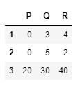
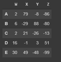
Pandas allow the conditional selection similar to NumPy, for the examples of this we will use the DataFrame:

print(df>0)
#       W       X       Y       Z
# A  True    True    False   False
# B  True    False   True    False
# C  True    True    False   False
# D  True    False   True    True
# E  True    True    False   False

print(df[df>0])
#    W   X      Y    Z
# A  2   79.0   NaN  NaN
# B  6   NaN    88.0 NaN
# C  2   21.0   NaN  NaN
# D  16  NaN    3.0  51.0
# E  30  49.0   NaN  NaN

More examples

print(df['X']>0)
#A     True
#B    False
#C     True
#D    False
#E     True
#Name: X, dtype: bool

print(df[df['X']>0])
#   W   X   Y   Z
#A  2   79  -8  -86
#C  2   21  -26 -13
#E  30  49  -48 -99

print(df[df['X']>0]['Y'])
#A    -8
#C   -26
#E   -48
#Name: Y, dtype: int64

print(df[df['X']>0][['Y','Z']])
#    Y    Z
#A  -8  -86
#C  -26 -13
#E  -48 -99

If we want to use more than one conditional we can us binary operator like "|" or "&".

print(df[(df['W']>0) & (df['Y'] > 1)])
#   W   X   Y   Z
#B  6   -29 88  -80
#D  16  -1  3   51

More about index

We can reset the index, this means change the index selected ( in this case the letters A to E) for the number (starting in 0), lit copy if this change is not reassigned it wont take place.

Again we start with

# Reset to default 0,1...n index
df.reset_index()

#   index   W   X   Y   Z
#0  A   2   79  -8  -86
#1  B   6   -29 88  -80
#2  C   2   21  -26 -13
#3  D   16  -1  3   51
#4  E   30  49  -48 -99

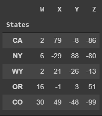
now we can create new index, in the following example we will create a new index starting from a string

newid = 'CA NY WY OR CO'.split()
df['states'] = newind
df = df.set_index('states')

Summaries

THere are 3 methods we can use to get information about the data in the DataFrames they are:

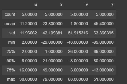
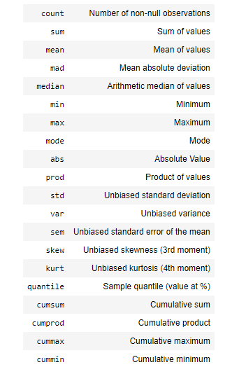
• describe() which will give a statistic description of the values

df.describe()

• info() overall description of what is in the table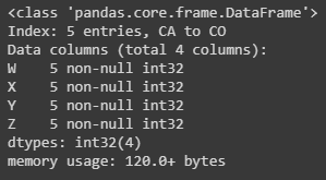

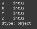
  df.info()
  

  

• dtypes() to display the data type

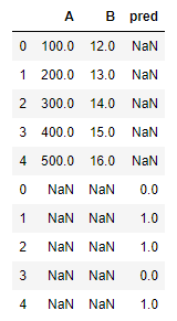
Missing Data

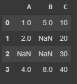
There are some methods in POandas that allow you to handle missing data in the DataFrames or series,

First lets create a new DataFrame with missing data

import numpy as np
import pandas as pd

df = pd.DataFrame({'A':[1,2,np,nan,4],
                    'B':[5,np,nan,np,nan,8],
                    'C':[10,20,30,40]})

Removing missing data

To remove horizontally

df.dropna()
#   A   B   C
#0  1.0 5.0 10
#3  4.0 8.0 40

To do it Vertically

df.dropna(axis=1)
#    C
# 0 10
# 1 20
# 2 30
# 3 40

Threshold

We can set a threshold for each column or row, if the row or column has equal or more of specific number of non-NaN

df.dropna(thresh=2)
#   A   B   C
#0  1.0 5.0 10
#1  2.0 NaN 20
#3  4.0 8.0 40

Filling missing data

Now to fill the empty values we can use fillna(value=0) using as a argument for the parameter value either a string of an integer

df.fillna(value='FILL VALUE')

#   A           B           C
#0  1           5           10
#1  2           FILL VALUE  20
#2  FILL VALUE  FILL VALUE  30
#3  4           8           40

df['A'].fillna(value=0)

#0    1.0
#1    2.0
#2    0.0
#3    4.0
#Name: A, dtype: float64

df['A'].fillna(df['A'].mean())

#0    1.000000
#1    2.000000
#2    2.333333
#3    4.000000
#Name: A, dtype: float64

Groupby

the Method groupby() allow me to group different rows and call other functions ( aggregate functions)

first we will need to choose the column that we are going to use as a categorical column, which is the same that we are going to use with groupby, Second choose the aggregated function (e.g. max,min, mean, std, etc...)

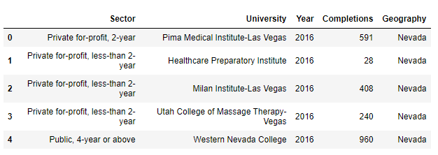
let make and example, we are going to read a file called "Universities.csv" and use the column 'Year' to group.

import pandas as pd

#read the csv file
df = pd.read_csv('Universities.cvs')

#now we can show the first rows
df.head()

#now group by Year
df.groupby('Year')
#<pandas.core.groupby.generic.DataFrameGroupBy object at 0x00000220102EC048>
# the groupby will be a DataFrame

# we can use the the aggregated
df.groupby('Year'),mean()

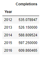
As well as the groupby the result of df.groupby('Year').mean() will be a DataFrame as well.

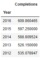
we can sort the results of mean()

df.groupby('Year').mean().sort_index(ascending=False)

Groupby by multiple columns

We can make the grouping by multiple columns we just need to

df.groupby(['Year','Sector']).mean()

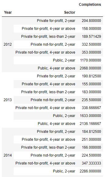
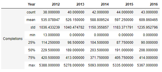
Now we are going to use describe() which will give use information about this dataFrame, but we will combine it with transpose() so we can change the columns for the rows and display it in a more readable way ( we are going to use just groupby with "Year")

df.groupby('Year').describe().transpose()

Operations

There are a set of operation that are useful but don't fall in a specific category

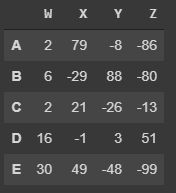
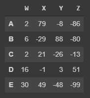
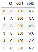
for the next operation we will create the following DataFrame:

import pandas as pd

df_one = pd.DataFrame({'k1':['A','A','B','B','C','C'],'col1':[100,200,300,300,400,500],'col2':['NY','CA','WA','WA','AK','NV']})

Unique Values

• Get the unique values.

  df_one['col2'].unique()
  # array(['NY', 'CA', 'WA', 'AK', 'NV'], dtype=object)
  

• Get number of unique values.

  df_one['col2'].nunique()
  # 5
  

• Count and Get the number of times a value is repeated

  df_one['col2'].value_counts()
  # WA    2
  # CA    1
  # NV    1
  # NY    1
  # AK    1
  

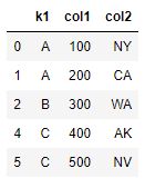
• To remove duplicated rows

df_one['col2'].drop_duplicates()

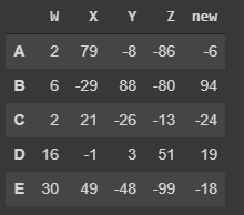
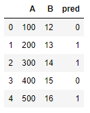
Create new Columns with Operations and Functions

def_one['New col'] = df_one['col1'] * 10

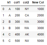
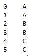
or we can use the method apply() and pass a customize function as a parameter

def grab_first_letter(state):
    return state[0]


df_one['first letter'] = df_one['col2'].apply(grab_first_letter)

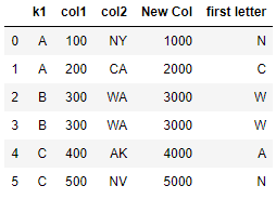
Be aware that we are not making a call of the function grab_first_letter(), there is not "()".

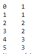
Mapping

now we are going to mapped some value to other lets check the column "k1"

df_one['k1'].map({'A':1,'B':2,'C':3})

Sorting, min, max, columns and index

to get the max, min or their positions we use:

• To find max value: df_one['col1'].max()
• The index of the max value: df_one['col1'].idxmax()
• To find min value: df_one['col1'].min()
• The index of the min value: df_one['col1'].idxmin()
• Now for sorting: df_one.sort_values('col2')

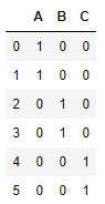
Concatenate DataFrames and Dummy variables

to concatenate we need to be careful in which axis we want to work with,

features = pd.DataFrame({'A':[100,200,300,400,500],
                        'B':[12,13,14,15,16]})
predictions = pd.DataFrame({'pred':[0,1,1,0,1]})

pd.concat([features,predictions])

pd.concat([features,predictions],axis=1)

for the dummy variables, first, we are going to change the name of the columns

df_one.columns = ['C1','C2','C3','C4','C5','C6']

later we can make the dummy variable

pd.get_dummies(df_one['C1'])

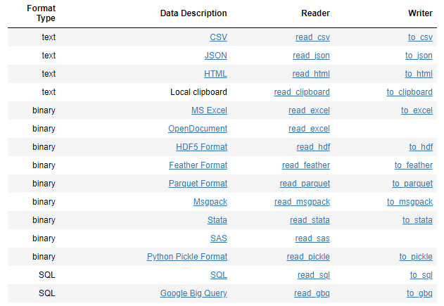
Data input and Data Output

for more detailed information of the different type of files and please visit the pandas documentation

CSV

To be able to read this type of files we need two additional libraries:

• xlrd ( pip install xlrd ).
• openpyxl ( pip install openpyxl).

for reading CSV:

df = pd.read_csv('example.csv')

for the Output

df = df.to_csv('example.csv', index = False)

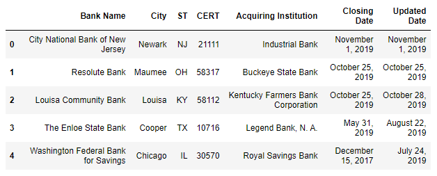
HTML

Pandas is able to read table tabs of the HTML (if the firewall allow pandas to read the HTML) but it is necessary to add the following libraries:

• lxml ( pip install lxml).
• html5lib (pip install html5lib).
• beautifulsoap4 ( pip install beautifulsoap4).

for the input, the read_html function willl read tables of the webpage and return a list of DataFrame object:

tables = pd.read_html('http://www.fdic.gov/bank/individual/failed/banklist.html')
tables[0].head()