Numpy Crash course

This notes are notes for the Numpy crash course.

Numpy is a linear library for Python, it is an essential building block for other PyData ecosystem ( Pandas, scipy, scikit-lean, etc)

Using NumPy

Normally numpy is import as np

import numpy as np

NumPy Arrays

NumPy came in vector and matrices, Vectors are 1 dimension, matrix are 2D dimensions.

Create NumPy Arrays

we can create an array from a python list

my_list = [1,2,3]
np.array(my_list)
# array([1, 2, 3])

and can be a list of list as well

my_matrix = [[1,2,3],[4,5,6],[7,8,9]]
np.array(my_matrix)
#array([[1, 2, 3],
#       [4, 5, 6],
#       [7, 8, 9]])

Build-in Methods

arange

Return evenly spaced value within a given interval

np.arange(0,10)
# array([0,1,2,3,4,5,6,7,8,9])
np.arange(0,11,2)
# array([0, 2, 4, 6, 8, 10])

zeros and ones

Generate vectors or matrix of zeros or ones

np.zero(3)
# array([0. , 0. , 0.])

np.zero((5,5))
# array([[0., 0., 0., 0., 0.],
#        [0., 0., 0., 0., 0.],
#        [0., 0., 0., 0., 0.],
#        [0., 0., 0., 0., 0.],
#        [0., 0., 0., 0., 0.]])

np.ones(3)
# array([1., 1., 1.])

np.ones((3,3))
# array([[1., 1., 1.],
#       [1., 1., 1.],
#       [1., 1., 1.]])

linspace

Return evenly spaced numbers over a specific interval

np.linspace(0,10,3)
# array([0., 5., 10.])

np.linspace(0,5,20)
# array([0.        , 0.26315789, 0.52631579, 0.78947368, 1.05263158,
#       1.31578947, 1.57894737, 1.84210526, 2.10526316, 2.36842105,
#       2.63157895, 2.89473684, 3.15789474, 3.42105263, 3.68421053,
#       3.94736842, 4.21052632, 4.47368421, 4.73684211, 5.        ])

#Note that .linspace() includes the stop value. To obtain an array of common fractions, increase the number of items:

np.linspace(0,5,21)
# array([0.  , 0.25, 0.5 , 0.75, 1.  , 1.25, 1.5 , 1.75, 2.  , 2.25, 2.5 ,
#       2.75, 3.  , 3.25, 3.5 , 3.75, 4.  , 4.25, 4.5 , 4.75, 5.  ])

eye identity matrix

Create a identity matrix

np.eye(4)
# array([[1., 0., 0., 0.],
#       [0., 1., 0., 0.],
#       [0., 0., 1., 0.],
#       [0., 0., 0., 1.]])

Random

Here some of the ways we can create random numbers

rand

Creates an array of the given shape with random uniform distribution over [0,1)

np.random.rand(2)
# array([0.37065108, 0.89813878])
np.random.rand(5,5)
# array([[0.03932992, 0.80719137, 0.50145497, 0.68816102, 0.1216304 ],
#       [0.44966851, 0.92572848, 0.70802042, 0.10461719, 0.53768331],
#       [0.12201904, 0.5940684 , 0.89979774, 0.3424078 , 0.77421593],
#       [0.53191409, 0.0112285 , 0.3989947 , 0.8946967 , 0.2497392 ],
#       [0.5814085 , 0.37563686, 0.15266028, 0.42948309, 0.26434141]])

randint

This generate a integer from low (inclusive) to high (exclusive)

np.random.randint(1,100)
#61
np.random.randint(1,100,10)
# array([39, 50, 72, 18,27, 59, 15, 97, 11, 14])

seed

It is use to create a random state that can be reproducible, i means, the result will be the same everything we use the same seed

np.random.seed(42)
np.random.rand(4)
# array([0.37454012, 0.95071431, 0.73199394, 0.59865848])

np.random.seed(42)
np.random.rand(4)
# array([0.37454012, 0.95071431, 0.73199394, 0.59865848])

Array Attributes and Methods

To explain the attributes and methods we need to create a vector and matrix

arr = np.arange(25)
# array([ 0,  1,  2,  3,  4,  5,  6,  7,  8,  9, 10, 11, 12, 13, 14, 15, 16,
#       17, 18, 19, 20, 21, 22, 23, 24])
ranarr = np.random.randint(0,50,10)
# array([38, 18, 22, 10, 10, 23, 35, 39, 23,  2])

Reshape - reshape

Return the same data of the vector or matrix but in a different shape

arr.reshape(5,5)
# array([[ 0,  1,  2,  3,  4],
#       [ 5,  6,  7,  8,  9],
#       [10, 11, 12, 13, 14],
#       [15, 16, 17, 18, 19],
#       [20, 21, 22, 23, 24]])

max, min, argmax, argmin - max,min,argmax,argmin

Let start with ranarr

ranarr = np.random.randint(0,50,10)
# array([38, 18, 22, 10, 10, 23, 35, 39, 23,  2])

the maximum number in the array

ranarr.max()
# 39

the index of this maximum number

ranarr.argmax()
# 7

now for the minimum

ranarr.min()
# 2
ranarr.argmin()
# 9

Shape - shape

shape is an attribute and not a method

# Vector
arr.shape
#(25,)

# Notice the two sets of brackets
arr.reshape(1,25)
# array([[ 0,  1,  2,  3,  4,  5,  6,  7,  8,  9, 10, 11, 12, 13, 14, 15,
#        16, 17, 18, 19, 20, 21, 22, 23, 24]])

arr.reshape(1,25).shape
# (1, 25)

arr.reshape(25,1)
#array([[ 0],
#       [ 1],
#       [ 2],
#       [ 3],
#       [ 4],
#       [ 5],
#       [ 6],
#       [ 7],
#       [ 8],
#       [ 9],
#       [10],
#       [11],
#       [12],
#       [13],
#       [14],
#       [15],
#       [16],
#       [17],
#       [18],
#       [19],
#       [20],
#       [21],
#       [22],
#       [23],
#       [24]])

arr.reshape(25,1).shape
# (25, 1)

dtype

In order to know the data type of the object

arr.dtype
# dtype('int32')

arr2 = np.array([1.2, 3.4, 5.6])
arr2.dtype

#dtype('float64')

Numpy Indexing and Selection

To select an item in the array we can use a syntax similar to the one use to pick up elements of a list, in the following example we will:

1. Create an array

import numpy as np#create an array
arr = np.arange(0,11)

2. Select a single element

arr[7]
#7

3. Select a range of elements

arr[0:5]
#array([0,1,2,3,4])\

Broadcasting

The differences between Python list and Numpy arrays can be simplify as; python list you can only reassign values to part of the list with the same size and shape, if you want to replace X number of elements you will need to pass in a new x element list, this is explain better with an example.

In the example: 1. Create an array. 2. Slice part of the array. 3. We will change the sliced array. 4. Display the original array.

Notice the elements of the array, that belong to the sliced array, were change. This is because the data is not copied in order to avoid memory problems.

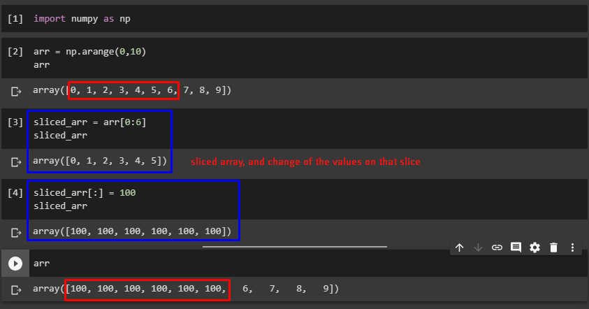
import numpy as np
#create an array
arr= np.arange(0,10)
#slice the array
sliced_arr = arr[0:6]
#change the values in the slice
sliced_arr[:] = 100
# print the original array to show the changes
print(arr)
#array([100, 100, 100, 100, 100, 100,   6,   7,   8,   9])

If you want to make a copy of the array you can use copy() like new_arr = arr.copy()

Indexing 2d arrays (matrices)

The syntax will be arr_2d[row][col] or arr_2d[row,col], the latter the most common used.

1. Create the matrix

import numpy as np
arr_2d = np.arange([5,10,15],[20,25,30],[35,40,45])

2. Select base in index

a row

arr_2d[1]
#array([20,25,30])

a value

arr_2d[1][0]
#20

3. select a matrix inside the matrix

arr_2d[:2,1:] # top right corner
# array([25,30],
#       [40,45])

Conditional selection

We can select elements of the arrays base in a condition, let say we want to know what elements are bigger than 4.

import numpy as np
arr = np.arange(0,10)
print(arr>4)
#array([False, False, False, False,  True,  True,  True,  True,  True,
#        True])

we can save this array of boolean values and use it to slice or select elements of the original array base in this condition

bool_arr = arr>4
arr[bool_arr]
# array([ 5,  6,  7,  8,  9, 10])
arr[arr>4]
# array([ 5,  6,  7,  8,  9, 10])

Operations

Arithmetic

Numpy allows operation including matrix with matrix and scalar with matrix.

1. Addition, multiplication , subtraction and division

import numpy as np

arr = np.arange(0,10)
arr
#array([0, 1, 2, 3, 4, 5, 6, 7, 8, 9])

#addition
arr + arr
#array([ 0,  2,  4,  6,  8, 10, 12, 14, 16, 18])

# Multiplication
arr * arr
#array([ 0,  1,  4,  9, 16, 25, 36, 49, 64, 81])

#Subtraction
arr - arr
#array([0, 0, 0, 0, 0, 0, 0, 0, 0, 0])

#Division
arr/arr
#array([nan,  1.,  1.,  1.,  1.,  1.,  1.,  1.,  1.,  1.])

numpy will notify us when the division is not possible or the division by 0

1/arr
#array([       inf, 1.        , 0.5       , 0.33333333, 0.25      ,
#       0.2       , 0.16666667, 0.14285714, 0.125     , 0.11111111])

and we have the exponential as well

arr**3
#array([  0,   1,   8,  27,  64, 125, 216, 343, 512, 729])

Universal Array function

With Numpy we can perform different function to the matrices, square root, logarithmic and geometric functions.

 np.sqrt(arr)
 #array([0.        , 1.        , 1.41421356, 1.73205081, 2.        ,
 #      2.23606798, 2.44948974, 2.64575131, 2.82842712, 3.        ])

# Exponential (e^)
np.exp(arr)
#array([1.00000000e+00, 2.71828183e+00, 7.38905610e+00, 2.00855369e+01,
#       5.45981500e+01, 1.48413159e+02, 4.03428793e+02, 1.09663316e+03,
#       2.98095799e+03, 8.10308393e+03])

#Trigonometric
np.sin(arr)
#array([ 0.        ,  0.84147098,  0.90929743,  0.14112001, -0.7568025 ,
#       -0.95892427, -0.2794155 ,  0.6569866 ,  0.98935825,  0.41211849])

#Natural Logarithm
np.log(arr)
#array([      -inf, 0.        , 0.69314718, 1.09861229, 1.38629436,
#       1.60943791, 1.79175947, 1.94591015, 2.07944154, 2.19722458])

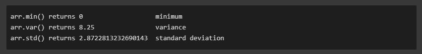
Statistics

as an example of the statistic function that can be perform in numpy we have sum, mean and max

arr = np.arange(0,10)

arr.sum()
#45

arr.mean()
#4.5

arr.max()
#9

and other examples of statistic functions

Axis Logic

Wen we work with 2D arrays (Matrix) the array term , axis 0 is the vertical axis ( rows ), and axis 1 is the horizontal ( columns )

so let do sum on the 0 axis, basically sum all the elements vertically, it make sense after the code.

arr_2d = np.array([[1,2,3,4],[5,6,7,8],[9,10,11,12]])
arr_2d
#array([[ 1,  2,  3,  4],
#       [ 5,  6,  7,  8],
#       [ 9, 10, 11, 12]])

arr_2d.sum(axis=0)
#array([15, 18, 21, 24])
#[(1+5+9), (2+6+10), (3+7+11), (4+8+12)]

arr_2d.sum(axis=1)
#array([10, 26, 42])