Images and Numpy

in this case i will use Jupyter lab for the code, so the code in this document will have some parts specific for Jupyter lab, additionally the course gave me some images that i will use, so i will refer to those images too.

First we need to remember that python alone is not able to handle the images, it needs a library to do so, in this case we are going to use PLI or pillow

Get the image with Python

so in this case we are going to use the function open() to get the image, in the next step we will transfor the image in a Numpy array

import numpy as np
import mathplotlib.pyplot as plt
%matplotlib inline #--> this line is just for Jupyter Lab, in order to disply images

We imported the mathplotlib in order to display the image in the Jypyter lab, now we are going to import Image from PIL

from PIL import Image

next, we need to load the image

import numpy as np
import mathplotlib.pyplot as plt
%matplotlib inline #--> this line is just for Jupyter Lab, in order to display images
from PIL import Image

pic = Image.open('path-to/the-image.jpg')

Transform the image to a Numpy array

At this point the image is load but it

pic = Image.open('Computer-Vision-with-Python/DATA/00-puppy.jpg')
type(pic)
# PIL.JpegImagePlugin.JpegImageFile

in this case we have a Jpeg Image file, now we need to transform it to Numpy array

pic_arr = np.asarray(pic)
type(pic_arr)
# numpy.ndarray

with the function called asarray we transform this image field to a Numpy array.

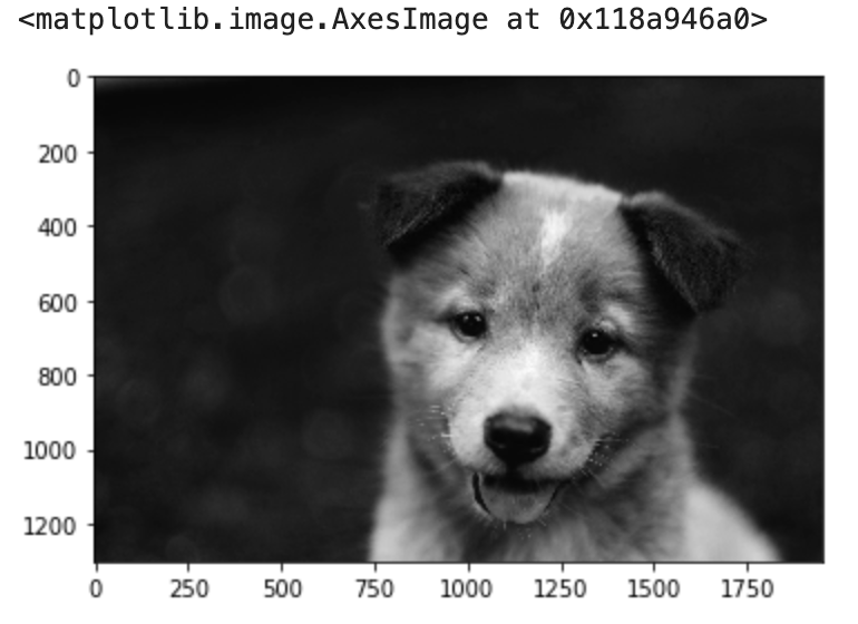
Display the image with imshow

pic_arr.shape
(1300, 1950, 3)

in this case we have an array with 1300x1950 with 3 channels, this means, that the image is a color image, so, now lest display this array as an image

 plt.imshow(pic_arr)

you will get

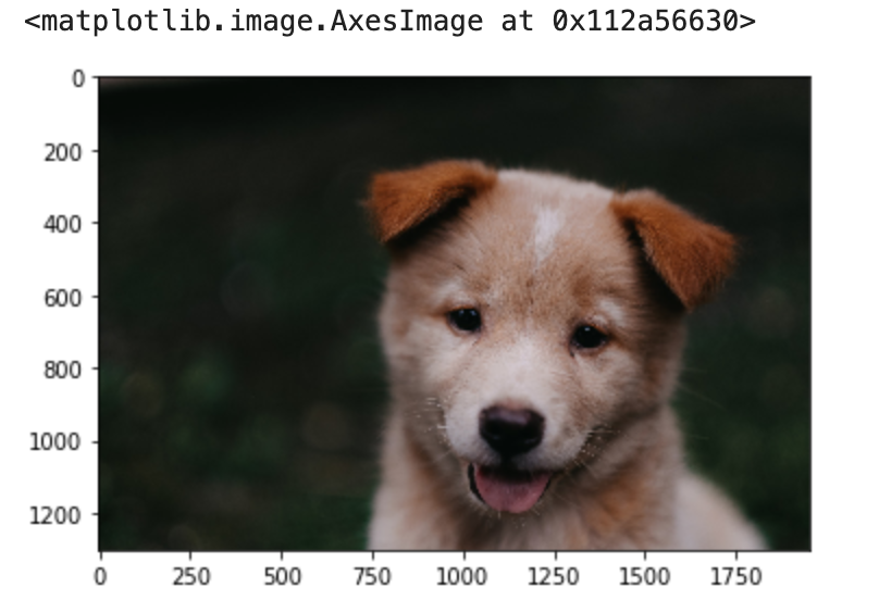
plt.imshow(image_numpy_array) the plt.imshow is a special function from matplotlib use to display images that are in a Numpy array format.

Color mapping one channel to grayscale

We know that the image is a color image, that means, it has 3 channels, and we confirm this when we ask for its shape (pic_arr.shape) which result was (1300, 1950, 3), so first we are going to make a copy and later slice the one of the channels

pic_red = pic_arr.copy()
pic_red = pic_red[:,:,0]
plt.imshow(pic_red)

the result will be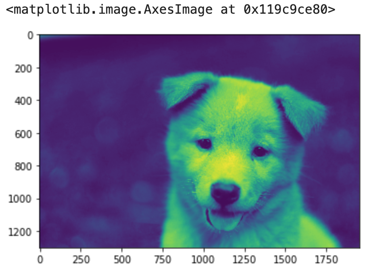

pic_red.shape
# (1300, 1950)

how it looks is due to how , matplotlib handle the colors, in this case is displaying the image in a format that will be special for people with an specific color blindness.

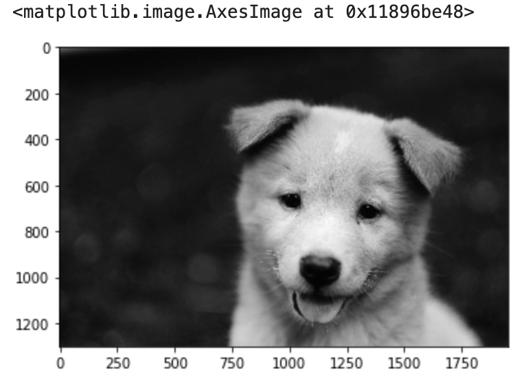
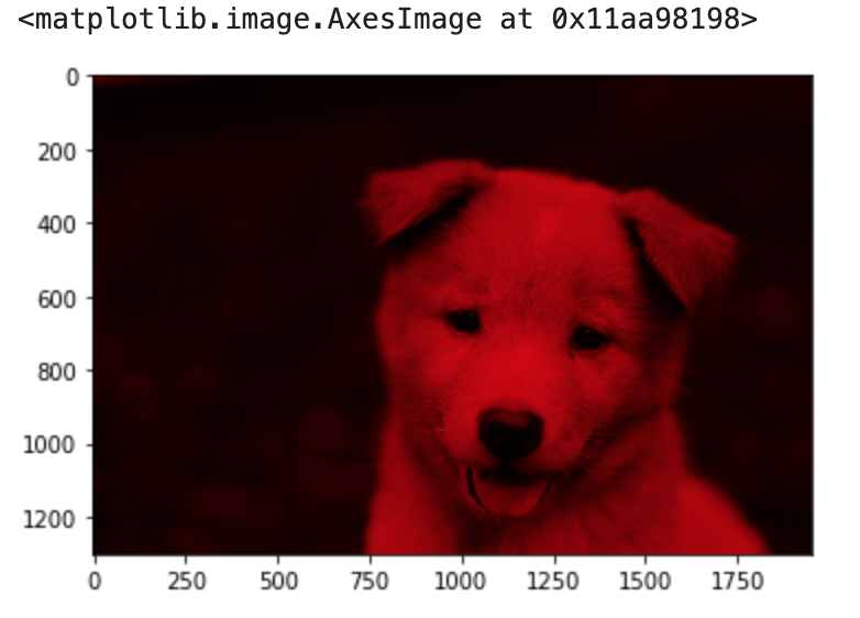
We can display the image in gray scale, but the question will be, Gray?, we are going to map the color red to a gray-scale

plt.imshow(pic_red, cmap='gray')

we can see the difference when we get the other colors, green and blue

Blue

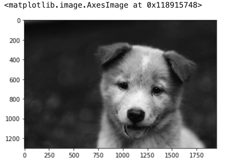pic_green = pic_arr.copy()
pic_green = pic_green[:,:,1]
plt.imshow(pic_green, cmap = 'gray')

Green

pic_blue = pic_arr.copy()
pic_blue = pic_blue[:,:,2]
plt.imshow(pic_blue, cmap = 'gray')

now comparing the 3 images

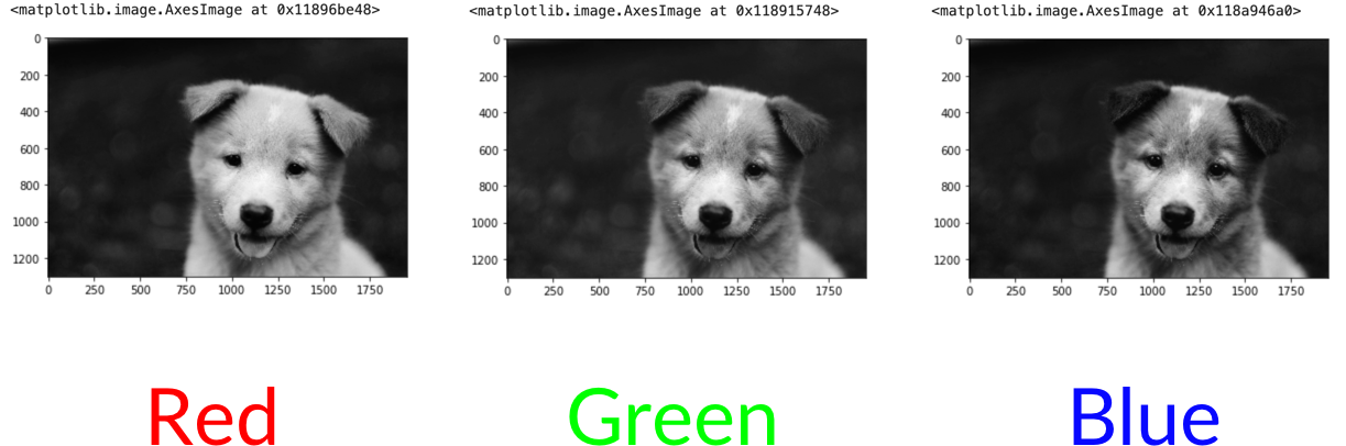
Then we can say that in each channel, the closest is the pixel to the color of the channel, closest to 255, and closest to white, for example, in the image of the red channel, the parts of the picture that are more white means that they contain more red, and those that are black means that contain no red. This is mapping the color to a gray scale, but we are not removing the contribution of the colors.

Removing contribution of the channels

In this part we are going to remove the contribution of the channels Blue and Green so we can have an image with the tree channels but with 0 contribution in two of those channels.

pic_red_real= pic_arr.copy()
pic_red_real[:,:,1] = 0
pic_red_real[:,:,2] = 0
plt.imshow(pic_red_real)

and if we check the shape

pic_red_real.shape
# (1300, 1950, 3)